Building a Movie Review Analysis - Jupyter Notebook and Flask

The job of a film critic is a highly responsible job. These days, people have become smart enough to read or watch a movie review before investing their money in a ticket. The lot depends on the movie reviews nowadays and therefore they are important.

Films reviews provide advance information about the film before it reaches the final audience. Generally, the critics see the film before the actual release or on the day of release and they review it based on what they feel. A good film critic talks about various aspects of film making like cinematography, acting, sound design, music, etc. without giving any spoilers so that audience can decide whether they want to spend money on a film or not.

To begin we first install all python libraries needed, in this project we will use the following libraries Pandas, NumPy, Matplotlib, Seaborn, Naïve Bayes, Sklearn, Logistic Regression, Random Forest Classifier, Pickle and etc. In order to make all libraries available in our Jupyter Notebook, we will first install

Visit Web App   http://sentiment.rogerkoranteng.com/

Download a copy of my Book - Beginner's Guide To Data Science

https://drive.google.com/file/d/1JaEsRa7ThL6D_x-VocMpwnxlfr8hpBZh/view

!install pandas
!install numpy
!install matplotlib
!install seaborn

After successfully installing all python libraries we can go ahead and import them

to Jupyter

import pandas as pd
import numpy as np
import matplotlib.pyplot as plt
import seaborn as sns
%matplotlib inline
import warnings
warnings.filterwarnings("ignore")

To make data available to Jupyter we will import our data

df = pd.read_csv("imdb_dataset.csv")

To check whether data has been imported properly, we will print the first 10 columns with the

head function

df.head(10)

In every data science training project its essential that we split our data into a train and test set, appropriately data is split into 80 percent for training and 20 percent for test

from sklearn.model_selection import train_test_split
X_train, X_test, y_train, y_test = train_test_split(df['review'], df['sentiment'], \
                                                    test_size=0.1, random_state=0)

Finally, after splitting our data set we can proceed to import our model

Random Forest Classifier

rom sklearn.ensemble import RandomForestClassifier
rf = RandomForestClassifier(n_estimators=1000)
rf.fit(trainVector, y_train)
predictions = rf.predict(testVector)
modelEvaluation(predictions)

Output

Accuracy on validation set: 0.7640

AUC score : 0.7641

Classification report : 
               precision    recall  f1-score   support

           0       0.75      0.78      0.77       249
           1       0.77      0.75      0.76       251

    accuracy                           0.76       500
   macro avg       0.76      0.76      0.76       500
weighted avg       0.76      0.76      0.76       500


Confusion Matrix : 
 [[194  55]
 [ 63 188]]

For a better model performance we will use LSTM which allows us to use Keras API to

compile and fit the model

The video below demonstrate how the application works

from keras.preprocessing import sequence
from keras.utils import np_utils
from keras.models import Sequential
from keras.layers.core import Dense, Dropout, Activation, Lambda
from keras.layers.embeddings import Embedding
from keras.layers.recurrent import LSTM, SimpleRNN, GRU
from keras.preprocessing.text import Tokenizer
from collections import defaultdict
from keras.layers.convolutional import Convolution1D
from keras import backend as K
from keras.layers.embeddings import Embedding

epoch = 6
batch_size = 62
maxlen = 200
classes = 4
words = 40000

Convert X_Train and X_Test to 2D tensor

2D tensors or two-dimensional tensors are the equivalent of two-dimensional metrics. A two-dimensional tensor, like a two-dimensional metric, has $n$ rows and columns. As an example, consider a grayscale image, which is a two-dimensional matrix of numeric values known as pixels.

tokenizer = Tokenizer(nb_words=top_words) #only consider top 20000 words in the corpse
tokenizer.fit_on_texts(X_train)

sequences_train = tokenizer.texts_to_sequences(X_train)
sequences_test = tokenizer.texts_to_sequences(X_test)

X_train_seq = sequence.pad_sequences(sequences_train, maxlen=maxlen)
X_test_seq = sequence.pad_sequences(sequences_test, maxlen=maxlen)

One hot encoding

y_train_seq = np_utils.to_categorical(y_train, nb_classes)
y_test_seq = np_utils.to_categorical(y_test, nb_classes)

print('X_train shape:', X_train_seq.shape)
print("========================================")
print('X_test shape:', X_test_seq.shape)
print("========================================")
print('y_train shape:', y_train_seq.shape)
print("========================================")
print('y_test shape:', y_test_seq.shape)
print("========================================")

output

X_train shape: (4500, 200)
========================================
X_test shape: (500, 200)
========================================
y_train shape: (4500, 4)
========================================
y_test shape: (500, 4)
========================================

model1 = Sequential()
model1.add(Embedding(top_words, 128, dropout=0.2))
model1.add(LSTM(128, dropout_W=0.2, dropout_U=0.2)) 
model1.add(Dense(nb_classes))
model1.add(Activation('softmax'))
model1.summary()

Model: "sequential_1"
_________________________________________________________________
Layer (type)                 Output Shape              Param #   
=================================================================
embedding_1 (Embedding)      (None, None, 128)         5120000   
_________________________________________________________________
lstm_1 (LSTM)                (None, 128)               131584    
_________________________________________________________________
dense_1 (Dense)              (None, 4)                 516       
_________________________________________________________________
activation_1 (Activation)    (None, 4)                 0         
=================================================================
Total params: 5,252,100
Trainable params: 5,252,100
Non-trainable params: 0

model1.compile(loss='binary_crossentropy',
              optimizer='adam',
              metrics=['accuracy'])

model1.fit(X_train_seq, y_train_seq, batch_size=batch_size, nb_epoch=nb_epoch, verbose=1)

# Model evluation
score = model1.evaluate(X_test_seq, y_test_seq, batch_size=batch_size)
print('Test loss : {:.4f}'.format(score[0]))
print('Test accuracy : {:.4f}'.format(score[1]))

Epoch 1/6
4500/4500 [==============================] - 22s 5ms/step - loss: 0.3760 - accuracy: 0.7594
Epoch 2/6
4500/4500 [==============================] - 24s 5ms/step - loss: 0.2857 - accuracy: 0.8577
Epoch 3/6
4500/4500 [==============================] - 24s 5ms/step - loss: 0.1591 - accuracy: 0.9347
Epoch 4/6
4500/4500 [==============================] - 24s 5ms/step - loss: 0.0838 - accuracy: 0.9699
Epoch 5/6
4500/4500 [==============================] - 24s 5ms/step - loss: 0.0385 - accuracy: 0.9874
Epoch 6/6
4500/4500 [==============================] - 24s 5ms/step - loss: 0.0225 - accuracy: 0.9925
500/500 [==============================] - 1s 1ms/step
Test loss : 0.4559
Test accuracy : 0.8750

len(X_train_seq),len(y_train_seq)

print("Size of weight matrix in the embedding layer : ", \
      model1.layers[0].get_weights()[0].shape)

# get weight matrix of the hidden layer
print("Size of weight matrix in the hidden layer : ", \
      model1.layers[1].get_weights()[0].shape)

# get weight matrix of the output layer
print("Size of weight matrix in the output layer : ", \
      model1.layers[2].get_weights()[0].shape)

import pickle
pickle.dump(model1,open('model1.pkl','wb'))

Section B

In this section, we will build our Flask App to integrate our trained model

from flask import Flask,render_template,url_for,request
import numpy as np
import pickle
import pandas as pd
import flasgger
from flasgger import Swagger
from sklearn.feature_extraction.text import CountVectorizer
from sklearn.naive_bayes import MultinomialNB
#from sklearn.externals import joblib

app=Flask(__name__)
Swagger(app)

mnb = pickle.load(open('model_imdb.pkl','rb'))
countVect = pickle.load(open('countVect.pkl','rb'))

@app.route('/').
def home():
    return render_template('home.html')

@app.route('/sentiment',methods=['POST'])
def predict():

    if request.method == 'POST':
        Reviews = request.form['Reviews']
        data = [Reviews]
        vect = countVect.transform(data).toarray()
        my_prediction = mnb.predict(vect)
    return render_template('result.html',prediction = my_prediction)



if __name__ == '__main__':
    app.run(debug=True)
    

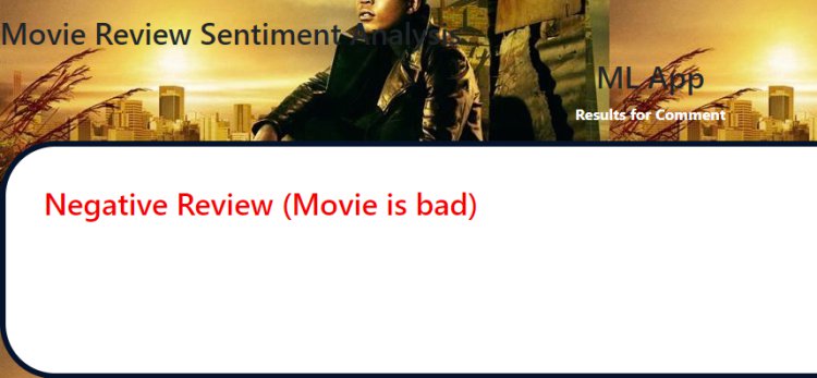
In the images below I would demonstrate how the application works

Example One

I would use the statements "This movie has got bad sound quality" 

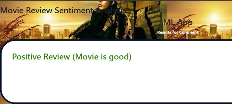
Example Two

I would use the statements "This movie has got good sound quality" 

Visit Web App   http://sentiment.rogerkoranteng.com/

Visit my Github page on   Click Here  

https://github.com/rogerkorantenng/Movie-Review-Sentinel