


Using the Sentinel L1C satellite to monitor deforestation in wild life reserves with your Jupyter Notebook
This blog seeks to take you through all the steps to using images obtained from the Sentinel satellite to monitor deforestation
In 2010, Ghana had 7.00Mha of natural forest, extending over 30% of its land area. In 2021, it lost 101kha of natural forest, equivalent to 62.9Mt of CO₂ emissions. This has lead to the drying up of headwaters of water bodies which supplies water to major cities in the country. As a result of logging activities in our forest, Ghana has had a higher percentage of deforestation since the 90's.

Sentinel-2 (an Earth observation mission from the Copernicus Programme that systematically acquires optical imagery at high spatial resolution (10 m to 60 m) over land and coastal waters.) using the bands from 1,2,3,4,5,6,7,8,8a,9,10,11,12 we will compare images from Mole National Park in the Savannah region of Ghana and Ankasa Game Reserve in the Western Region of Ghan
Steps used to build it
- Download and Import all python libraries
- We used "http://bboxfinder.com" to obtain the co-ordinates of Mole National Park and Ankasa Game Forest by passing it's xMin, yMin, xMax and yMax through bboxfinder's search_bbox function.
- We used the search_time_interval python function to determine the time interval.
- To obtain the tile_info for the specified period of time, we used wfs_iterator to extract a unique tile info for each tile.
- Next, we converted each tile_id obtained into a tile_name which was accessed from the s3 bucket.
- For clearer results, we chose the tile_id with the least cloud cover.
- Next, we selected bands 'B01','B02','B03','B04','B07','B08','B8A', 'B10','B11','B12'
- We specified our download folders for both Mole National Park(Mole_Data) and Ankasa Game Reserves(Ankasa_Data).
- We then requested for the data using the request.save_data function.
- Next, we triggered the download and specified the bands we want to download.
- After downloading the images to our folder, we plotted our image using matplotlib.
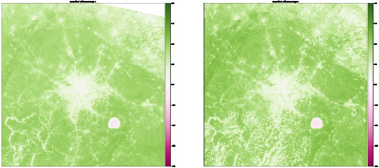
- To highlight on the area affected most we imported rasterio and used the GeoTIFF feature to check the vegetation of the selected area.
- Band 4 and Band 8 was used because we were checking for the vegetation view.
- Finally, we plotted our obtained image.
The video below takes you through all the steps used
Steps explained in Details
Stage One: Install and Import required libraries
In this step we will install all python libraries that will be needed. The first will be to install the Pandas python library followed by NumPy, Geopandas, Matplotlib and the list goes on. After installing our libraries, we can then import previously installed libraries
%pip install pandas
%pip install numpy
%pip install geopandas
%pip install shapely
%pip install matplotlib
%pip install plotly_express
%pip install sentinelhub
%pip install rasterio
%pip install earthpyname: geo-data
%pip install utils
!pip install sentinelhub==3.4.1
import pandas as pd
import numpy as np
import geopandas as gpd
from shapely.geometry import Point
import matplotlib
import matplotlib.pyplot as plt
import folium
import plotly_express as px
import os
import warnings
import datetime
warnings.filterwarnings('ignore')
After all libraries have been successfully installed, we will also import some libraries from the Sentinel Hub
from sentinelhub import (
    MimeType,
    CRS,
    BBox,
    SentinelHubRequest,
    SentinelHubDownloadClient,
    DataCollection,
    bbox_to_dimensions,
    DownloadRequest
)
The next most important thing to do is configure your AWS Secret Key and Sentinel Instance ID
To do this we will head over to AWS IAM console, set up our secret keys and save
Head over Sentinel Hub, sign up and go to the configuration utility to access your keys
#Input instance id and client id from the sentinel hub
#input aws iAM keys for access to my aws account
from sentinelhub import SHConfig

config = SHConfig()

config.instance_id = '' #instance id
config.sh_client_id = ''  #sentinel hub client id
config.sh_client_secret = ''  #sentinel hub secret
config.aws_access_key_id = ''  #aws access key
config.aws_secret_access_key = '' #aws secret key
Save your configuration
#Save configuration
config.save()
Finally we import WFS to allows us perform some data manipulations
#Input WFS to allow us to perform some data manipulation on different geographical locations
from sentinelhub import WebFeatureService, BBox, CRS, DataCollection, SHConfig
if config.instance_id == '':
    print("Warning! To use WFS functionality, please configure the `instance_id`.")
Stage Two: Using Bbox finder to specify your Longitute and Latitude
A bounding box (abbreviated bbox) is an area defined by two longitudes and two latitudes in which:
Latitude is a decimal number ranging from -90.0 to 90.0.
Longitude is a decimal number ranging from -180.0 to 180.0.
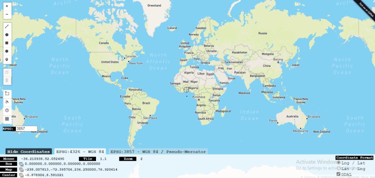
Log on to bboxfinder.com Bbox, and locate the area you would like to obtain the images from the satelitte.
In the code below I specified Mole National Park as our primary location
#Use Bbox to specify the geographical location of Mole National Park https://molenationalpark.org/
search_bbox = BBox(bbox=[-1.851196,9.264779,-1.788025,9.700935], crs=CRS.WGS84)
search_time_interval = ("2021-01-10T00:00:00", "2022-12-10T23:59:59")


wfs_iterator = WebFeatureService(
    search_bbox, search_time_interval, data_collection=DataCollection.SENTINEL2_L1C, maxcc=1.0, config=config
)

for tile_info in wfs_iterator:
    print(tile_info)
The first line search_bbox, allows us to specify our Longitude and Latitute, the proceeding line search_time_interval, allows us to specify the date and time period we want to retrieve the images.
Finally we can print our tiles
A tile obtained can be in the format below
{'type': 'Feature', 'geometry': {'type': 'MultiPolygon', 'crs': {'type': 'name', 'properties': {'name': 'urn:ogc:def:crs:EPSG::4326'}}, 'coordinates': [[[[-1.9246049674382728, 9.949669984838678], [-2.0897179274737763, 9.200678565551982], [-2.090331938754135, 8.957173405588467], [-1.0918256072464385, 8.953372194561377], [-1.0863496013234732, 9.94592425838906], [-1.9246049674382728, 9.949669984838678]]]]}, 'properties': {'id': 'S2B_OPER_MSI_L1C_TL_VGS2_20210111T123100_A020111_T30PXR_N02.09', 'date': '2021-01-11', 'time': '10:38:30', 'path': 's3://sentinel-s2-l1c/tiles/30/P/XR/2021/1/11/0', 'crs': 'EPSG:32630', 'mbr': '600000,990240 709800,1100040', 'cloudCoverPercentage': 5.34}}
Stage 3: Convert each tile_id obtained into a tile_name which was accessed from the s3 bucket
from sentinelhub import AwsTile

tile_id = 'S2A_OPER_MSI_L1C_TL_SGS__20200112T120158_A023800_T30NXN_N02.08'
tile_name, time, aws_index = AwsTile.tile_id_to_tile(tile_id)
tile_name, time, aws_index

tile_id2 = 'S2B_OPER_MSI_L1C_TL_SGS__20200117T121509_A014963_T30NXN_N02.08'
tile_name2, time2, aws_index2 = AwsTile.tile_id_to_tile(tile_id2)
tile_name2, time2, aws_index2
from sentinelhub import CRS, BBox, DataCollection, SHConfig, WebFeatureService

config = SHConfig()

if config.instance_id == "":
    print("Warning! To use WFS functionality, please configure the `instance_id`.")
Stage 4: Select the appropraite bands needed
The Sentinel-2 satellites each carry a single multi-spectral instrument (MSI) with 13 spectral channels in the visible/near infrared (VNIR) and short wave infrared spectral range (SWIR). Within the 13 bands, the 10 meter spatial resolution allows for continued collaboration with the SPOT-5 and Landsat-8 missions, with the core focus being land classification
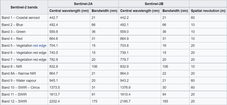
In this stage I will select the bands needed, B01,B02,B03,B04,B07,B08,B8A, B10,B11,B12
| B01 | Band 1 |
| B02 | Band 2 |
| B03 | Band 3 |
| B04 | Band 4 |
| B07 | Band 7 |
| B08 | Band 8 |
| B08A | Band 8A |
| B10 | Band 10 |
| B11 | Band 11 |
| B12 | Band 12 |
#Import the type of bands needed and specify our folder Data to store the data
warnings.simplefilter("ignore", UserWarning)
from sentinelhub import AwsTileRequest

bands = ['B01','B02','B03','B04','B07','B08','B8A', 'B10','B11','B12']
metafiles = ['tileInfo', 'preview', 'qi/MSK_CLOUDS_B00']
data_folder = './Mole_Data'
In the code above we imported AwsTileRequest and specified the bands we needed to collect images from
The meta files specifies what info we want to retrieve along side our data, in the third line we will create a folder named Mole_Data
Stage 4: Trigger our download
After successfully creating our folder Mole_Data we will then trigger our download
#Trigger the download to create the folder Data
request = AwsTileRequest(
    tile=tile_name,
    time=time,
    aws_index=aws_index,
    bands=bands,
    metafiles=metafiles,
    data_folder=data_folder,
    data_collection=DataCollection.SENTINEL2_L1C
)

request.save_data()


request2 = AwsTileRequest(
    tile=tile_name2,
    time=time2,
    aws_index=aws_index2,
    bands=bands,
    metafiles=metafiles,
    data_folder=data_folder,
    data_collection=DataCollection.SENTINEL2_L1C
)

request2.save_data()
We can then go ahead to download our data
#Download data one
data_list = request.get_data(redownload=True)

p_b01,p_b02,p_b03,p_b04,p_b07,p_b08,p_b8a,p_b10,p_b11,p_b12,p_tile_info, p_preview, p_cloud_mask = data_list
#Download data two
data_list2 = request2.get_data(redownload=True)
p_b01_2,p_b02_2,p_b03_2,p_b04_2,p_b07_2,p_b08_2,p_b8a_2,p_b10_2,p_b11_2,p_b12_2,p_tile_info_2, p_preview_2, p_cloud_mask_2 = data_list2
After all images have been successfully downloaded, we will go ahead to plot our images using Matplotlib
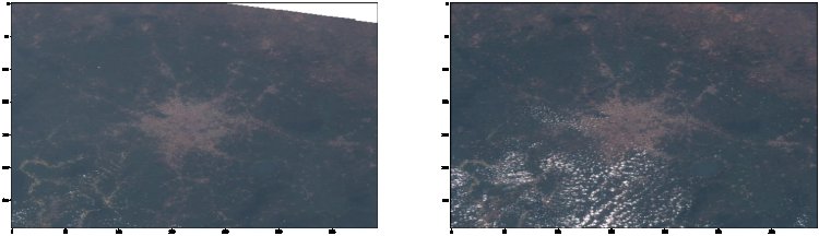
What's Your Reaction?