Using a probabilistic approach, we would use previous earthquake occurances and apply advanced statistical models to forecast possible future occurance. This is not scientifically proven but uses a supervised machine learning technique to forecast

Visit App Here

Download a copy of my Book - Beginner's Guide To Data Science Here

Downlaod Link

http://earthquake.rogerkoranteng.com/

Extreme Gradient Boosting (XGBoost) is a scalable distributed gradient-boosted decision tree machine learning library. Predicting earthquakes is nearly impossible because earthquakes are unpredictable in terms of where they will strike next. In this project, I will use XGBoost, a supervised machine learning technique, to forecast earthquakes based on historical data. How XGBoost works

Why was XGBoost prefered for this project?

XGBoost is efficient, accurate and fast. It has a capacity to do powerful computation on a single machine. In this blog I would take you through the steps used in building a flask app trained with XGBoost to use live data from United States Geological Survey. To begin this project in Jupyter Notebook, I would install and import all python libraries needed. Some libraries which will be required in this project are Pandas, NumPy, Matplot;ib, XGBoost and Sklearn

import pandas as pd
import numpy as np
import matplotlib.pyplot as plt
from sklearn import preprocessing;
from sklearn import model_selection;
from sklearn import linear_model;
from sklearn.model_selection import train_test_split
from sklearn.datasets import make_classification
from sklearn.model_selection import GridSearchCV
from sklearn.metrics import roc_curve
from sklearn.metrics import auc
from sklearn.metrics import roc_auc_score
from sklearn.metrics import recall_score
from sklearn.metrics import confusion_matrix
%matplotlib inline
import xgboost as xgb

After successfully installing all libraries, I would then make the data avaliable to Jupyter Notebook. Our data will be named EarthQuake.csv and Earthquake_predict.csv

data = pd.read_csv('EarthQuake.csv')

data_predict = pd.read_csv('Earthquake_predict.csv')

To verify whether our data has been properly imported, we would check the first five rows with the python function .head() 

data.head()

The next stage is to determine the correletion between the attributes in our dataset with the corr()

corr_matrix = data.corr()

corr_matrix['mag_outcome'].sort_values(ascending=False)

Next, we would remove some attributes to make the data more clean and precise.

To make some data avaliable for testing, we would then split data into 80% for training and 20% for testing

attributes = [f for f in list(data) if f not in ['date', 'lon_box_mean',
 'lat_box_mean', 'mag_outcome', 'mag', 'place',
 'combo_box_mean',  'latitude',
 'longitude']]

# splitting training and testing dataset 80% and 20% respectively
X_train, X_test, y_train, y_test = train_test_split(data[attributes],
                     data['mag_outcome'], test_size=0.2, random_state=42)

Once data has been split into our train set and test set, we can then fit our data into our model XGBoost and calculate for the AUC. AUC which stands for Area Under the Curve, measures the two-dimensional area underneath the entire ROC curve. The best score can span from 0.8 - 0.9 which translate to 80% - 90%.

To tune our hyperparameters we would use Grid Search, Grid Search uses a different combination of all the specified hyperparameters and their values and calculates the performance for each combination and selects the best value for the hyperparameters. This makes the processing time-consuming and expensive based on the number of hyperparameters involved.

dtrain = xgb.DMatrix(X_train[attributes], label=y_train)
dtest = xgb.DMatrix(X_test[attributes], label=y_test)


param = {
        'objective': 'binary:logistic',
        'booster': 'gbtree',
        'eval_metric': 'auc',
        'max_depth': 6,  # the maximum depth of each tree
        'eta': 0.003,  # the training step for each iteration
        'silent': 1}  # logging mode - quiet}  # the number of classes that exist in this datset
num_round = 5000  # the number of training iterations    
bst = xgb.train(param, dtrain, num_round)
preds = bst.predict(dtest)

print (roc_auc_score(y_test, preds))
fpr, tpr, _ = roc_curve(y_test, preds)
roc_auc = auc(fpr, tpr)
print('AUC:', np.round(roc_auc,4))

ypred_bst = np.array(bst.predict(dtest,ntree_limit=bst.best_iteration))
ypred_bst  = ypred_bst > 0.5
ypred_bst = ypred_bst.astype(int)  

This gives us an outcome and AUC ;

0.9883235758947253

AUC: 0.9883

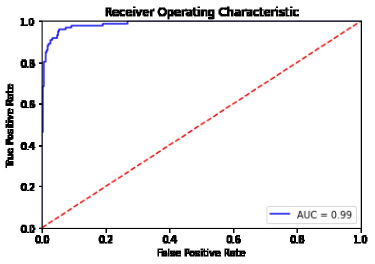
Next we would plot our Receiving Operating Characteristics, An ROC curve (receiver operating characteristic curve) is a graph showing the performance of a classification model at all classification thresholds. This curve plots two parameters: Learn more about AUC and RUC here or For beginner's visit here

• True Positive Rate
• False Positive Rate

To get a more detailed understanding, we would plot our results using Matplotlib

plt.title('Receiver Operating Characteristic')
plt.plot(fpr, tpr, 'b', label = 'AUC = %0.2f' % roc_auc)
plt.legend(loc = 'lower right')
plt.plot([0, 1], [0, 1],'r--')
plt.xlim([0, 1])
plt.ylim([0, 1])
plt.ylabel('True Positive Rate')
plt.xlabel('False Positive Rate')
plt.show()

Using Confusion Matrix and Recall

A confusion matrix is a summary of prediction results on a classification problem. The number of correct and incorrect predictions are summarized with count values and broken down by each class.

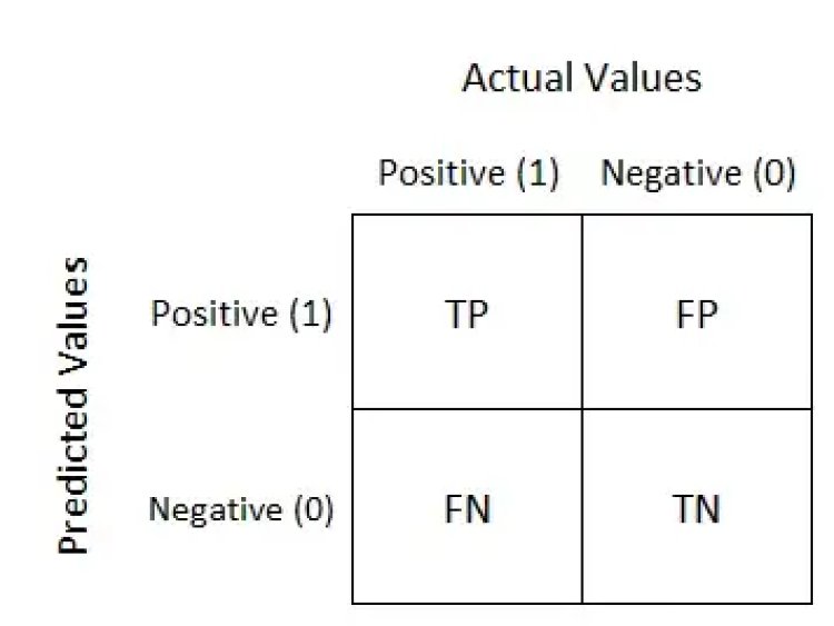
The recall is calculated as the proportion of Positive samples that were correctly classified as Positive to the total number of Positive samples. The recall factor assesses the model's ability to identify positive samples. The recall is calculated as the proportion of Positive samples that were correctly classified as Positive to the total number of Positive samples. The recall factor assesses the model's ability to identify positive samples.

print("Confusion Matrix: \n",confusion_matrix(y_test,ypred_bst))
print("\nRecall 'TP/TP+FN' = ", recall_score(y_test,ypred_bst))

Confusion Matrix: 

 [[2413    24]

 [  20      81]]

Recall  'TP/TP+FN' =  0.801980198019802

Section Two

Building a python flask app which will receive live data and use XGBoost to forecast future occurances

How the App Works

The app takes real time data from the United States Geological Survey and apply XGBoost technique to each loop, this app is build to predict within a five days range

First we would import the Flask library and instantiate the app function with (__name__), to make our libraries accessible to the pp we would import the following libraries (render_template, numpy, pandas, XGBoost and etc)

Next, we would set our Global variable as  earthquake_live and set app to predict in a five days rands

from flask import Flask

app = Flask(__name__)

from flask import render_template, flash, request
import logging, io, base64, os, datetime
from datetime import datetime
from datetime import timedelta
import numpy as np
import xgboost as xgb
import pandas as pd

# Variables(Global)
earthquake_live = None
days_out_to_predict = 5

Next we would create a python function Prepare_earthquake_date_and_model, this function will take how many days to predict and would extract live data from the USGS 

def prepare_earthquake_data_and_model(days_out_to_predict = 5, max_depth=3, eta=0.1):

data = pd.read_csv('https://earthquake.usgs.gov/earthquakes/feed/v1.0/summary/all_month.csv')
    data = data.sort_values('time', ascending=True)

We would then truncate time from datetime

    data['date'] = data['time'].str[0:10]

To get away with uneccessary columns in order to prevent noise, we would keep only a section of the data

 data = data[['date', 'latitude', 'longitude', 'depth', 'mag', 'place']]
    temp_data = data['place'].str.split(', ', expand=True) 
    data['place'] = temp_data[1]
    data = data[['date', 'latitude', 'longitude', 'depth', 'mag', 'place']]

Get access to full code here

By Roger Obeng Koranteng

Conclusion and Remarks

Some major take aways from this project are;

• According to USGS predicting earthqaukes are nearly impossibe
• This project used past earthquake occurances to forcast possible occurances using XGBoost and data from the UGSC